ITCS’2012 in Cambridge, MA

November 29th, 2011

Since everything I write now seems to provide an occasion for bitter controversy, I’ll be curious to learn whose sensibilities I inadvertently offended by posting the following announcement for next year’s ITCS conference. -SA


Dear Theorists:

As you know the third Innovation in Theoretical Computer Science Conference will be held in Cambridge this January:  http://research.microsoft.com/en-us/um/newengland/events/itcs2012/.

REGISTRATION IS NOW OPEN and THE PROGRAM IS ONLINE.

In addition to the program, there are going to be a few novelties that we would like to point out to you.

1. GRADUATING BITS

In one session of the conference, students graduating this academic year (as well as researchers completing their postdoc this academic year) will be given few minutes to present themselves and their work.

The presentations will be grouped by University, in alphabetic order.

We hope this will give all of us an opportunity to have a synopsis of the great work being done by the “graduating” members of our community.

In order to speak in this special session, please send an email at  silvio.itcs12@gmail.com by DECEMBER 15.

Registration fees will be waived for presenters at Graduating Bits 2012.

If you/your students are graduating this year, or you plan to hire this year, we are encourage to attend ITCS 2012!

2. COMMUNITY BUILDING

To strengthen our (legendary!) friendship and collaboration, we will treat you to a PLAY BACK show: an improvisational theater where OUR actors will bring to life YOUR stories.

3. CHAIR RANTS

In addition to the chair of each session introducing the speakers and coauthors of the session (who will then introduce themselves and their coauthors), our chairs will provide us with their insights on the papers in their sessions.

We look forward to seeing all of you in Cambridge very soon!

All the Best

Shafi Goldwasser, Silvio Micali, and Yael Tauman Kalai

2.373

November 28th, 2011

For twenty years, the fastest known algorithm to multiply two n-by-n matrices, due to Coppersmith and Winograd, took a leisurely O(n2.376) steps.   Last year, though, in his PhD thesis, Andrew Stothers gave an improvement to O(n2.374) steps.  And today,  Virginia Vassilevska Williams of Berkeley and Stanford, released a paper that gives a general methodology for analyzing Coppersmith-Winograd-type algorithms, and that improves the matrix-multiplication time to a lightning-fast O(n2.373) steps.  (Virgi’s work was independent of Stothers’, though she credits him and applies an idea of his to simplify her proof.)  Full disclosure: I actually knew a month ago that this was coming—I had a hell of a time keeping the secret.  I’d recommend that you get started memorizing “ω<2.373,” but as Russell Impagliazzo points out in the comments, the exponent might get lowered again in short order.  Huge congratulations to Virgi and to Andrew for this breakthrough!


Update (Nov. 30): Last night I received an extremely gracious email from Andrew Stothers, which he’s given me permission to summarize here.  In the email, Andrew expressed how excited he was about Virgi’s new result, apologized for the confusion he caused by not mentioning his improvement to ω until page 71 of his thesis (he says he doesn’t know why he did it), and said that he meant to publish a paper, but was prevented from doing so by health and job issues.  He also said that he didn’t take issue with anything I wrote here, except that I mistakenly referred to him as Andy rather than Andrew.  In response, I congratulated Andrew on his achievement; expressed how happy I was that—ironically—his work is now finally getting some of the attention that it deserves; and promised to buy him a beer when and if I’m ever in Edinburgh, a city I’ve always wanted to visit.  (On the other hand, I warned Andrew that his LinkedIn profile, which unselfconsciously mentions improvements to his Word and Excel skills as one of the benefits of his PhD research breaching the Coppersmith-Winograd barrier, might have earned him a place in scientific folklore forever!)

In summary, I now see Andrew as an extraordinarily nice fellow who had some bad luck and—most conspicuously—a lack of good advice from people around him.  I do stand by the points that I was originally trying to make:

(a) that this tangled situation shouldn’t in any way detract from Virgi’s fantastic achievement, which (except for a simplification, as she discusses) must be considered completely independent of Andrew’s, and

(b) that there’s indeed an important cautionary lesson for students here, about adequately publicizing your work (yes, there’s a happy medium, between hiring a PR firm to wage a viral marketing campaign and burying your solution to a longstanding open problem so far in the body of your PhD thesis that even world experts in the subject who read your thesis will miss it).

On the other hand, I hereby apologize for anything I said that could even be perceived as slighting Andrew, his important work, or his motives.


Another Update: On the third hand, if you’re one of the commenters whose beef is not about attribution, but about the entire concept of using a CS theory blog to “promote” major milestones in CS theory (like the breaking of the Coppersmith-Winograd barrier), then I apologize for absolutely nothing.  Go read an economics or physics blog; I understand that those are entirely hype-free.  Better yet, go to hell.

The quantum state cannot be interpreted as something other than a quantum state

November 19th, 2011

Lots of people asked me to comment on a much-discussed new preprint by Matthew Pusey, Jonathan Barrett, and Terry Rudolph (henceforth PBR), “The quantum state cannot be interpreted statistically”.  (See here for an effusive Nature News article, here for the predictable Slashdot confusion-fest, here for a related Cosmic Variance guest post by David Wallace, and here for a spiteful rant by Lubos Motl that hilariously misunderstands the new result as “anti-quantum-mechanics.”)

I recommend reading the preprint if you haven’t done so yet; it should only take an hour.  PBR’s main result reminds me a little of the No-Cloning Theorem: it’s a profound triviality, something that most people who thought about quantum mechanics already knew, but probably didn’t know they knew.  (Some people are even making comparisons to Bell’s Theorem, but to me, the PBR result lacks the same surprise factor.)

To understand the new result, the first question we should ask is, what exactly do PBR mean by a quantum state being “statistically interpretable”?  Strangely, PBR spend barely a paragraph justifying their answer to this central question—but it’s easy enough to explain what their answer is.  Basically, PBR call something “statistical” if two people, who live in the same universe but have different information, could rationally disagree about it.  (They put it differently, but I’m pretty sure that’s what they mean.)  As for what “rational” means, all we’ll need to know is that a rational person can never assign a probability of 0 to something that will actually happen.

To illustrate, suppose a coin is flipped, and you (but not I) get a tip from a reliable source that the coin probably landed heads.  Then you and I will describe the coin using different probability distributions, but neither of us will be “wrong” or “irrational”, given the information we have.

In quantum mechanics, mixed states—the most general type of state—have exactly the same observer-relative property.  That isn’t surprising, since mixed states include classical probability distributions as a special case.  As I understand it, it’s this property of mixed states, more than anything else, that’s encouraged many people (especially in and around the Perimeter Institute) to chant slogans like “quantum states are states of knowledge, not states of nature.”

By contrast, pure states—states with perfect quantum coherence—seem intuitively much more “objective.”  Concretely, suppose I describe a physical system using a pure state |ψ>, and you describe the same system using a different pure state |φ>≠|ψ>.  Then it seems obvious that at least one of us has to be flat-out wrong, our confidence misplaced!  In other words, at least one of us should’ve assigned a mixed state rather than a pure state.  The PBR result basically formalizes and confirms that intuition.

In the special case that |ψ> and |φ> are orthogonal, the conclusion is obvious: we can just measure the system in a basis containing |ψ> and |φ>.  If we see outcome |ψ> then you’re “unmasked as irrational”, while if we see outcome |φ>, then I’m unmasked as irrational.

So let’s try a slightly more interesting, non-orthogonal example.  Suppose I describe a system S using the state |0>, while you describe it using the state |+>=(|0>+|1>)/√2.  Even then, there are some measurements and outcomes of those measurements that would clearly reveal one of us to have been irrational.  If we measure S in the {|0>,|1>} basis and get outcome |1>, then I was irrational.  If we measure in the {|+>,|->} basis (where |->=(|0>-|1>)/√2) and get outcome |->, then you were irrational.  Furthermore, if S is any qubit that obeys quantum mechanics, then it must have a decent probability either of returning outcome |1> when measured in the {|0>,|1>} basis, or of returning  outcome |-> when measured in the {|+>,|->} basis.

So, are we finished?  Well, PBR don’t discuss the simple argument above, but I assume they wouldn’t be satisfied with it.  In particular, they’d probably point out that it only unmasks one of us as irrational for some measurement outcomes—but who can say what the measurement outcome will be, especially if we don’t presuppose that the quantum state provides a complete description of reality?

What they want instead is a measurement that’s guaranteed to unmask someone as irrational, regardless of its outcome.  PBR show that this can be obtained, under one further assumption: that “rational beliefs behave well under tensor products.”  More concretely, suppose two people with different knowledge could rationally describe the same physical system S using different pure states, say |0> or |+> respectively.  Then if we consider a new system T, consisting of two independent copies of S, it should be rationally possible to describe T using any of the four states |0>|0>, |0>|+>, |+>|0>, or |+>|+>.  But now, PBR point out that there’s a 2-qubit orthonormal basis where the first vector is orthogonal to |0>|0>, the second vector is orthogonal to |0>|+>, the third vector is orthogonal to |+>|0>, and the fourth vector is orthogonal to |+>|+>.  So, if we measure in that basis, then someone will get unmasked as irrational regardless of the measurement result.

More generally, given any physical system S that you and I describe using different pure states |ψ> and |φ>, PBR define a new system T consisting of k independent copies of S, where k is inversely proportional to the angle between |ψ> and |φ>.  They then construct a projective measurement M on T such that, whichever of M’s 2k possible outcomes is observed, one of the 2k possible “tensor product beliefs” about T gets unmasked as irrational.  And that’s it (well, other than a generalization to the noisy case).

So, will this theorem finally end the century-old debate about the “reality” of quantum states—proving, with mathematical certitude, that the “ontic” camp was right and the “epistemic” camp was wrong?  To ask this question is to answer it.

(Clarification added for Lubos Motl and anyone else unwilling or unable to understand: The answer that I intended was “no.”  I don’t think the battle between the “ontic” and “epistemic” camps can ever be won, by its nature.  Nor has that particular battle ever interested me greatly, except insofar as some interesting mathematical results have come out of it.)

I expect that PBR’s philosophical opponents are already hard at work on a rebuttal paper: “The quantum state can too be interpreted statistically”, or even “The quantum state must be interpreted statistically.”

I expect the rebuttal to say that, yes, obviously two people can’t rationally assign different pure states to the same physical system—but only a fool would’ve ever thought otherwise, and that’s not what anyone ever meant by calling quantum states “statistical”, and anyway it’s beside the point, since pure states are just a degenerate special case of the more fundamental mixed states.

I expect the rebuttal to prove a contrary theorem, using a definition of the word “statistical” that subtly differs from PBRs.  I expect the difference between the two definitions to get buried somewhere in the body of the paper.

I expect the rebuttal to get blogged and Slashdotted.  I expect the Slashdot entry to get hundreds of comments taking strong sides, not one of which will acknowledge that the entire dispute hinges on the two camps’ differing definitions.

There’s an important lesson here for mathematicians, theoretical computer scientists, and analytic philosophers.  You want the kind of public interest in your work that the physicists enjoy?  Then stop being so goddamned precise with words!   The taxpayers who fund us—those who pay attention at all, that is—want a riveting show, a grand Einsteinian dispute about what is or isn’t real.  Who wants some mathematical spoilsport telling them: “Look, it all depends what you mean by ‘real.’  If you mean, uniquely determined by the complete state of the universe, and if you’re only talking about pure states, then…”

One final remark.  In their conclusion, PBR write:

… the quantum state has the striking property of being an exponentially complicated object.  Specifically, the number of real parameters needed to specify a quantum state is exponential in the number of systems n.  This has a consequence for classical simulation of quantum systems.  If a simulation is constrained by our assumptions—that is, if it must store in memory a state for a quantum system, with independent preparations assigned uncorrelated states—then it will need an amount of memory which is exponential in the number of quantum systems.

The above statement is certainly true, but it seems to me that it was already demonstrated—and much more convincingly—by (for example) the exponential separations between randomized and quantum communication complexities.

Simons Postdoctoral Fellowship Announcement

November 16th, 2011

The Theory of Computation (TOC) group at the Computer Science and Artificial Intelligence Laboratory (CSAIL) at MIT is seeking candidates for a post-doctoral position in the general area of the theory of computation. Applicants in all areas of theory are encouraged to apply, including (but not exclusive to) algorithms, complexity theory, combinatorial optimization, cryptography, distributed computing, game theory and computation, geometry, parallel computing, and quantum computing. This fellowship is made possible by a generous gift from the Simons Foundation.

The fellowship is a two year position, starting the summer or fall of 2012. The fellowship stipend is gauged to attract the highest caliber of applicants. Generous funds for scientific travel will be available for use at the fellow’s discretion. Fellows will be assigned a faculty member close to their research interests from the TOC group. Fellows will be encouraged (although not required) to teach a graduate seminar in their area of research.

Eligibility: Candidates must receive their PhD during the academic year immediately preceding that in which the fellowship would begin. There are no other restrictions based on nationality or any other basis.

Application Process: Candidate applications should include a description of professional interests and goals in research. Each application should include a curriculum vitae and the names and addresses of three or more individuals who will provide letters of recommendation. Letter writers should submit their letters directly to MIT to the address below. Please submit complete applications by January 6, 2012.

Address to submit application: All application materials and recommendation letters should be sent electronically to theory-postdoc@csail.mit.edu. The candidate’s name should be included in the subject line of the email. Alternatively, the materials can be also sent to the following address:
Simons Postdoctoral Fellowship, c/o Joanne Hanley
MIT Computer Science and Artificial Intelligence Laboratory
The Stata Center, Building 32-G672A
32 Vassar Street
Cambridge, MA 02139, USA.

The pedophile upper bound

November 14th, 2011

Lance Fortnow now has a post up about how wonderful Graham Spanier and Joe Paterno were, and how sorry he is to see them go.

For what it’s worth, I take an extremely different view.  I’d be thrilled to see the insane football culture at many American universities—the culture that Spanier and Paterno epitomized—brought down entirely, and some good might yet come of the Penn State tragedy if it helps that happen.  Football should be, as it is at MIT, one of many fine extracurricular activities that are available to interested students (alongside table tennis, glassblowing, robot-building…), rather than a primary reason for a university’s existence.

What’s interesting about the current scandal is precisely that it establishes some finite upper bound on what people will tolerate, and thereby illustrates just what it takes for the public to turn on its football heroes.  Certainly the destruction of academic standards doesn’t suffice (are you kidding?).  More interestingly, sexism, sexual harassment, and “ordinary” rape—offenses that have brought down countless male leaders in other fields—barely even make a dent in public consciousness where football stars are concerned.  With child rape, by contrast, one can actually find a non-negligible fraction of Americans who consider it comparable in gravity to football.  (Though, as the thousands of rioting Penn State students reminded us, that’s far from a universal opinion.)  Many commentators have already made the obvious comparisons to the Catholic Church’s abuse scandal, and the lesson for powerful institutions the world over is indeed a similar one: sure, imprison Galileo; by all means stay silent during the Holocaust; but don’t protect pedophiles—cross that line, and your otherwise all-forgiving constituents might finally turn on you.

I should say that both of my parents are Penn State grads, and they’re both disgusted right now with the culture of hooliganism there—a culture that was present even in the late 60s and early 70s, but that’s become much more dominant since.  To the many of you at Penn State who want a university that’s more than an adjunct to a literally-rapacious football program, you have this blog’s admiration and support as you struggle to reclaim your great institution.  Go for the touchdown—WOOOOO!

A hacker’s hacker

October 14th, 2011

Before someone else is “absolutely stunned” by my silence, let me hereby note with great sadness that Dennis Ritchie, principal designer of C, co-designer of Unix, Turing Award winner, and one of the world’s legendary computer scientists, has passed away at 70.  (See here for the NYT obituary, here for a more detailed ZDNet obituary, and here for Lance Fortnow’s encomium.)  I didn’t know Ritchie, but my father did, as a science and technology writer in the 70s and 80s.  And I often saw Ritchie in the halls when I spent several summers working at Bell Labs in college.  Mostly, though, I know Ritchie through the beautiful language he created.  It’s a testament to C’s elegance and simplicity that I, though extremely far from a hacker, find it almost as easy to express my thoughts in C as I do in my mother tongue, MS-DOS QBASIC.

Update (Oct. 26): AI pioneer and LISP inventor John McCarthy has passed away as well.  It’s been a tough month for computing revolutionaries.

What happened in the world this week

October 7th, 2011

A commenter named “Daniel Quilp” writes:

I am absolutely stunned that you have not posted an encomium to Steve Jobs.  You are a computer science professor.  Jobs was the most important innovator in the field.  You claim you want to reach out to the public but fail to take advantage of this opportunity.  Very sad, very disappointing.

Steve Jobs was indeed one of the great American innovators, and I was extremely sorry to hear about his passing.  I was riveted by the NYT obituary, from which I learned many facts about Jobs that I hadn’t known before.  Personally, I plan honor his memory by buying an iPhone 4S at the Apple Store near my apartment when it comes out on the 14th.  (I was debating between upgrading my 3GS to a 4S and switching to an Android, leaning toward 4S because of battery life.  The desire to honor the great man’s memory is what pushed me over the edge.)

As for why I didn’t write an encomium before: well, frankly, I don’t feel like being a theoretical computer scientist gives me any more of a “connection” to Steve Jobs than any of the hundreds of millions of people who use his products.  And when I do blog about world events, people often accuse me of jumping on a bandwagon and having nothing original to say, and tell me to stick to complexity theory.  That’s life as a blogger: not only is there nothing you can post, there’s nothing you can refrain from posting, that someone, somewhere, won’t be “absolutely stunned” by.

Even so, to anyone who was hurt or offended by my lack of a Steve Jobs post, I’m sorry.

And as long as I’m apologizing for silence about major news of the last week, I’m also sorry that I failed to congratulate the Royal Swedish Academy of Sciences for two truly magnificent decisions: first, awarding the Nobel Prize in Physics to Adam Riess, Saul Perlmutter, and Brian Schmidt for the discovery of the cosmic acceleration (see these two Cosmic Variance posts for more); second, awarding the Nobel Prize in Chemistry to Dan Shechtman for the discovery of quasicrystals.  If these two textbook-changing results don’t deserve Nobel Prizes, nothing does.

Since it’s Erev Yom Kippur, let me hereby repent for all of my countless mistakes, omissions, and lapses of judgment here at Shtetl-Optimized over the past year.  In the spirit of the “Kol Nidre” prayer, I also beg to be released from all survey articles that I promised to write, submissions that I promised to review, deadlines that I promised to meet, and emails that I promised to answer.  (Of course, if I were conventionally religious, I’d also have to repent for the very act of blogging on Yom Kippur.)

In Defense of Kolmogorov Complexity

September 27th, 2011

I got lots of useful and interesting feedback on my last post, though I also learned a valuable sociological lesson about the “two kinds of complexity theory”:

If you write about the kind of complexity theory that involves acronyms like NP, BQP/qpoly, and r.s.r., people will think the issues must be difficult and arcane, even if they’re not and can be understood with very little effort.  By contrast, if you write about the kind of complexity theory that can be illustrated using pictures of coffee cups, people will think the issues can be sorted out with 15 seconds of thought, and will happily propose ‘solutions’ that presuppose what needs to be explained, answer a different question, or fail in simple examples.

Seriously, a large number of commenters raised two important questions, which I’d like to address forthwith in this followup post.

The first question is why I omitted the notion of coarse-graining, which plays a central role in many accounts of entropy and complexity. The short answer is that I shouldn’t have omitted it.  In fact, as both Sean Carroll and Luca Trevisan (among others) quickly pointed out, one can tell a perfectly-reasonable story about the coffee cup by defining the “complextropy,” not in terms of sophistication, but in terms of the ordinary Kolmogorov complexity of a coarse-grained or “smeared-out” state.  If you define the complextropy that way, it should increase and then decrease as desired, and furthermore, it’s probably easier to prove that statement than using the sophistication-based definition (though both versions seem highly nontrivial to analyze).

So, the reason I turned to sophistication was basically just the mathematician’s instinct to situate every concept in the most general structure where that concept makes sense.  For example, why define “connectedness” for polygons in the Euclidean plane, if the concept makes sense for arbitrary topological spaces?  Or in our case, why define “complextropy” for dynamical systems that happen to have a spatial structure over which one can coarse-grain, if the concept also makes sense for arbitrary dynamical systems whose evolution is computable by an efficient algorithm?  Of course, [OPEN PROBLEM ALERT] it would be wonderful to know whether the two types of complextropy can be shown to be related for those dynamical systems for which they both make sense, or whether we can construct a convincing example that separates the two.

The second question is why I invoked Kolmogorov complexity in a discussion about thermodynamics: many people seemed to think that, by doing so, I was making some novel or controversial claim.  I wasn’t.  People like Charles Bennett, Seth Lloyd, and Wojciech Zurek have employed Kolmogorov complexity as a useful language for thermodynamics since the 1980s; I was simply following in their footsteps.  Basically, what Kolmogorov complexity lets you do is talk in a well-defined way about the “entropy” or “randomness” of an individual object, without reference to any ensemble from which the object was drawn.  And this is often extremely convenient: notice that Kolmogorov complexity snuck its way in even when we defined complextropy in terms of coarse-graining!

Of course, if our dynamical system is probabilistic, then we always can talk instead about the “actual” entropy; in that case Kolmogorov complexity basically just amounts to a shorthand.  On the other hand, if our system is deterministic, then talking about the (resource-bounded) Kolmogorov complexity seems essential—since in that case there’s no “true” randomness at all, only pseudorandomness.

But a few commenters went further, disparaging Kolmogorov complexity itself rather than just its application to a particular problem.  Here’s Shtetl-Optimized regular Raoul Ohio:

As usual, my DAH (Devil’s Advocate Hat) is on. This is convenient, because it allows you to comment on anything without doing the work to really understanding it. Thus I will proceed to disparage the notion of using Kolmogorov Complexity (KC) for anything but entertainment.

Math is a subject where a couple of interesting definitions and a few theorems can launch a subfield such as KC. I have never studied KC … but a brief reading of the subject suggests that it started as a joke, and today a lot of people are not in on it.

… the KC of things would change as knowledge in other fields progresses. For example, what is the KC of

δ = 4.66920160910299067185320382…, and

α = 2.502907875095892822283902873218… ?

These are Feigenbaum’s constants (http://en.wikipedia.org/wiki/Feigenbaum_constants). A couple of decades ago, no one knew anything about these numbers. With the concept of analyzing discrete dynamical systems by bifurcation diagrams in hand, these can be calculated with a short program. So, did KC(δ) and KC(α) drop dramatically 20 odd years ago?

…using KC reminds me of physics arguments that use the wave function for the universe. Sure, there must be such a thing, but it is hard to say much about it.

On the other side of the coin, the theorems and proofs in basic KC are rather similar to those in many fields of TCS, and many SO [Shtetl-Optimized] readers might not think of these as a joke…

My intuition is that the entire concept of KC is “ill-posed”, to borrow a term from PDE.

In the interest of “full disclosure”, I must mention that often in the past I have thought some topic was a bunch of hooey until I understood it, after which I thought is was profound, just like listening to Lenard [sic] Cohen.

I wrote a reply to Raoul, and then decided that it should go into a top-level post, for the edification of Kolmogorov-skeptics everywhere.  So without further ado:

Hi Raoul!

I think this is indeed one of those cases where if you understood more, you’d see why your dismissal was wrong. And unlike with (say) art, music, or religion, the reasons why your dismissal is wrong can be articulated in words!

Contrary to what you say, K(x) is not undefinable: I’ll define it right now, as the length of the shortest prefix-free program (in some fixed universal programming language) that prints x and then halts! K(x) is uncomputable, but that’s a very different issue, and something that’s been known since the 1960s.

Basically, what K(x) lets you do is give a clear, observer-independent meaning to the loose notion of there “not existing any patterns” in a string. Already from that statement, it’s obvious that K(x) is going to be hard to compute—for as you correctly point out, detecting the existence or nonexistence of patterns is hard!

(Though contrary to what you say, K(Feigenbaum’s constant) didn’t suddenly become small when Feigenbaum defined the constant, any more than 42038542390523059230 suddenly became composite when I wrote it down, probably for the first time in human history. Please don’t tell me that you make no distinction between mathematical truths and our knowledge of them!)

The key point is that, even without being able to compute K(x) for most x’s, you can still use the definition of K(x) to give meaning to hundreds of intuitions that otherwise would’ve remained forever at a handwaving level. For example:

“The overwhelming majority of strings are patternless.”

“If a short computer program outputs a patternless string, then it can only be doing so by generating the string randomly.”

And many, many less obvious statements—every one of which can be upgraded to a theorem once you have a mathematical definition of “patternlessness”!

Furthermore, the idea of Kolmogorov complexity has actually inspired some important experimental work! For example, if you could compute K, then you could compute the “similarity” between two DNA sequences D1 and D2 by comparing K(D1)+K(D2) to K(D1,D2).

Of course you can’t compute K, but you can compute useful upper bounds on it. For example, let G(x) be the number of bits in the gzip compression of the string x. Then comparing G(D1)+G(D2) to G(D1,D2) has turned out to be a very useful way to measure similarity between DNA sequences.

It’s really no different from how, even though we can never say whether a curve in the physical world is continuous or not (since that would require infinitely precise measurements), the mathematical theories dealing with continuity (e.g., calculus, topology) can still be applied in physics in all sorts of ways.

The First Law of Complexodynamics

September 23rd, 2011

A few weeks ago, I had the pleasure of attending FQXi’s Setting Time Aright conference, part of which took place on a cruise from Bergen, Norway to Copenhagen, Denmark.  (Why aren’t theoretical computer science conferences ever held on cruises?  If nothing else, it certainly cuts down on attendees sneaking away from the conference venue.)  This conference brought together physicists, cosmologists, philosophers, biologists, psychologists, and (for some strange reason) one quantum complexity blogger to pontificate about the existence, directionality, and nature of time.  If you want to know more about the conference, check out Sean Carroll’s Cosmic Variance posts here and here.

Sean also delivered the opening talk of the conference, during which (among other things) he asked a beautiful question: why does “complexity” or “interestingness” of physical systems seem to increase with time and then hit a maximum and decrease, in contrast to the entropy, which of course increases monotonically?

My purpose, in this post, is to sketch a possible answer to Sean’s question, drawing on concepts from Kolmogorov complexity.  If this answer has been suggested before, I’m sure someone will let me know in the comments section.

First, some background: we all know the Second Law, which says that the entropy of any closed system tends to increase with time until it reaches a maximum value.  Here “entropy” is slippery to define—we’ll come back to that later—but somehow measures how “random” or “generic” or “disordered” a system is.  As Sean points out in his wonderful book From Eternity to Here, the Second Law is almost a tautology: how could a system not tend to evolve to more “generic” configurations?  if it didn’t, those configurations wouldn’t be generic!  So the real question is not why the entropy is increasing, but why it was ever low to begin with.  In other words, why did the universe’s initial state at the big bang contain so much order for the universe’s subsequent evolution to destroy?  I won’t address that celebrated mystery in this post, but will simply take the low entropy of the initial state as given.

The point that interests us is this: even though isolated physical systems get monotonically more entropic, they don’t get monotonically more “complicated” or “interesting.”  Sean didn’t define what he meant by “complicated” or “interesting” here—indeed, defining those concepts was part of his challenge—but he illustrated what he had in mind with the example of a coffee cup.  Shamelessly ripping off his slides:

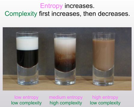
Entropy increases monotonically from left to right, but intuitively, the “complexity” seems highest in the middle picture: the one with all the tendrils of milk.  And same is true for the whole universe: shortly after the big bang, the universe was basically just a low-entropy soup of high-energy particles.  A googol years from now, after the last black holes have sputtered away in bursts of Hawking radiation, the universe will basically be just a high-entropy soup of low-energy particles.  But today, in between, the universe contains interesting structures such as galaxies and brains and hot-dog-shaped novelty vehicles.  We see the pattern:

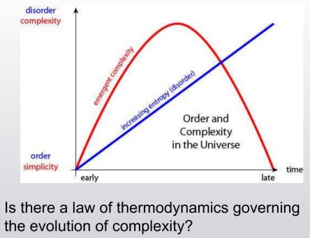
In answering Sean’s provocative question (whether there’s some “law of complexodynamics” that would explain his graph), it seems to me that the challenge is twofold:

  1. Come up with a plausible formal definition of “complexity.”
  2. Prove that the “complexity,” so defined, is large at intermediate times in natural model systems, despite being close to zero at the initial time and close to zero at late times.

To clarify: it’s not hard to explain, at least at a handwaving level, why the complexity should be close to zero at the initial time.  It’s because we assumed the entropy is close to zero, and entropy plausibly gives an upper bound on complexity.  Nor is it hard to explain why the complexity should be close to zero at late times: it’s because the system reaches equilibrium (i.e., something resembling the uniform distribution over all possible states), which we’re essentially defining to be simple.  At intermediate times, neither of those constraints is operative, and therefore the complexity could become large.  But does it become large?  How large?  How could we predict?  And what kind of “complexity” are we talking about, anyway?

After thinking on and off about these questions, I now conjecture that they can be answered using a notion called sophistication from the theory of Kolmogorov complexity.  Recall that the Kolmogorov complexity of a string x is the length of the shortest computer program that outputs x (in some Turing-universal programming language—the exact choice can be shown not to matter much).  Sophistication is a more … well, sophisticated concept, but we’ll get to that later.

As a first step, let’s use Kolmogorov complexity to define entropy.  Already it’s not quite obvious how to do that.  If you start, say, a cellular automaton, or a system of billiard balls, in some simple initial configuration, and then let it evolve for a while according to dynamical laws, visually it will look like the entropy is going up.  But if the system happens to be deterministic, then mathematically, its state can always be specified by giving (1) the initial state, and (2) the number of steps t it’s been run for.  The former takes a constant number of bits to specify (independent of t), while the latter takes log(t) bits.  It follows that, if we use Kolmogorov complexity as our stand-in for entropy, then the entropy can increase at most logarithmically with t—much slower than the linear or polynomial increase that we’d intuitively expect.

There are at least two ways to solve this problem.  The first is to consider probabilistic systems, rather than deterministic ones.  In the probabilistic case, the Kolmogorov complexity really does increase at a polynomial rate, as you’d expect.  The second solution is to replace the Kolmogorov complexity by the resource-bounded Kolmogorov complexity: the length of the shortest computer program that outputs the state in a short amount of time (or the size of the smallest, say, depth-3 circuit that outputs the state—for present purposes, it doesn’t even matter much what kind of resource bound we impose, as long as the bound is severe enough).  Even though there’s a computer program only log(t) bits long to compute the state of the system after t time steps, that program will typically use an amount of time that grows with t (or even faster), so if we rule out sufficiently complex programs, we can again get our program size to increase with t at a polynomial rate.

OK, that was entropy.  What about the thing Sean was calling “complexity”—which, to avoid confusion with other kinds of complexity, from now on I’m going to call “complextropy”?  For this, we’re going to need a cluster of related ideas that go under names like sophistication, Kolmogorov structure functions, and algorithmic statistics.  The backstory is that, in the 1970s (after introducing Kolmogorov complexity), Kolmogorov made an observation that was closely related to Sean’s observation above.  A uniformly random string, he said, has close-to-maximal Kolmogorov complexity, but it’s also one of the least “complex” or “interesting” strings imaginable.  After all, we can describe essentially everything you’d ever want to know about the string by saying “it’s random”!  But is there a way to formalize that intuition?  Indeed there is.

First, given a set S of n-bit strings, let K(S) be the number of bits in the shortest computer program that outputs the elements of S and then halts.  Also, given such a set S and an element x of S, let K(x|S) be the length of the shortest program that outputs x, given an oracle for testing membership in S.  Then we can let the sophistication of x, or Soph(x), be the smallest possible value of K(S), over all sets S such that

  1. x∈S and
  2. K(x|S) ≥ log2(|S|) – c, for some constant c.  (In other words, one can distill all the “nonrandom” information in x just by saying that x belongs that S.)

Intuitively, Soph(x) is the length of the shortest computer program that describes, not necessarily x itself, but a set S of which x is a “random” or “generic” member.  To illustrate, any string x with small Kolmogorov complexity has small sophistication, since we can let S be the singleton set {x}.  However, a uniformly-random string also has small sophistication, since we can let S be the set {0,1}n of all n-bit strings.  In fact, the question arises of whether there are any sophisticated strings!  Apparently, after Kolmogorov raised this question in the early 1980s, it was answered in the affirmative by Alexander Shen (for more, see this paper by Gács, Tromp, and Vitányi).  The construction is via a diagonalization argument that’s a bit too complicated to fit in this blog post.

But what does any of this have to do with coffee cups?  Well, at first glance, sophistication seems to have exactly the properties that we were looking for in a “complextropy” measure: it’s small for both simple strings and uniformly random strings, but large for strings in a weird third category of “neither simple nor random.”  Unfortunately, as we defined it above, sophistication still doesn’t do the job.  For deterministic systems, the problem is the same as the one pointed out earlier for Kolmogorov complexity: we can always describe the system’s state after t time steps by specifying the initial state, the transition rule, and t.  Therefore the sophistication can never exceed log(t)+c.  Even for probabilistic systems, though, we can specify the set S(t) of all possible states after t time steps by specifying the initial state, the probabilistic transition rule, and t.  And, at least assuming that the probability distribution over S(t) is uniform, by a simple counting argument the state after t steps will almost always be a “generic” element of S(t).  So again, the sophistication will almost never exceed log(t)+c.  (If the distribution over S(t) is nonuniform, then some technical further arguments are needed, which I omit.)

How can we fix this problem?  I think the key is to bring computational resource bounds into the picture.  (We already saw a hint of this in the discussion of entropy.)  In particular, suppose we define the complextropy of an n-bit string x to be something like the following:

the number of bits in the shortest computer program that runs in n log(n) time, and that outputs a nearly-uniform sample from a set S such that (i) x∈S, and (ii) any computer program that outputs x in n log(n) time, given an oracle that provides independent, uniform samples from S, has at least log2(|S|)-c bits, for some constant c.

Here n log(n) is just intended as a concrete example of a complexity bound: one could replace it with some other time bound, or a restriction to (say) constant-depth circuits or some other weak model of computation.  The motivation for the definition is that we want some “complextropy” measure that will assign a value close to 0 to the first and third coffee cups in the picture, but a large value to the second coffee cup.  And thus we consider the length of the shortest efficient computer program that outputs, not necessarily the target string x itself, but a sample from a probability distribution D such that x is not efficiently compressible with respect to D.  (In other words, x looks to any efficient algorithm like a “random” or “generic” sample from D.)

Note that it’s essential for this definition that we imposed a computational efficiency requirement in two places: on the sampling algorithm, and also on the algorithm that reconstructs x given the sampling oracle.  Without the first efficiency constraint, the complextropy could never exceed log(t)+c by the previous argument.  Meanwhile, without the second efficiency constraint, the complextropy would increase, but then it would probably keep right on increasing, for the following reason: a time-bounded sampling algorithm wouldn’t be able to sample from exactly the right set S, only a reasonable facsimile thereof, and a reconstruction algorithm with unlimited time could probably then use special properties of the target string x to reconstruct x with fewer than log2(|S|)-c bits.

But as long as we remember to put computational efficiency requirements on both algorithms, I conjecture that the complextropy will satisfy the “First Law of Complexodynamics,” exhibiting exactly the behavior that Sean wants: small for the initial state, large for intermediate states, then small again once the mixing has finished.  I don’t yet know how to prove this conjecture.  But crucially, it’s not a hopelessly open-ended question that one tosses out just to show how wide-ranging one’s thoughts are, but a relatively-bounded question about which actual theorems could be proved and actual papers published.

If you want to do so, the first step will be to “instantiate” everything I said above with a particular model system and particular resource constraints.  One good choice could be a discretized “coffee cup,” consisting of a 2D array of black and white pixels (the “coffee” and “milk”), which are initially in separated components and then subject to random nearest-neighbor mixing dynamics.  (E.g., at each time step, we pick an adjacent coffee pixel and milk pixel uniformly at random, and swap the two.)  Can we show that for such a system, the complextropy becomes large at intermediate times (intuitively, because of the need to specify the irregular boundaries between the regions of all-black pixels, all-white pixels, and mixed black-and-white pixels)?

One could try to show such a statement either theoretically or empirically.  Theoretically, I have no idea where to begin in proving it, despite a clear intuition that such a statement should hold: let me toss it out as a wonderful (I think) open problem!  At an empirical level, one could simply try to plot the complextropy in some simulated system, like the discrete coffee cup, and show that it has the predicted small-large-small behavior.   One obvious difficulty here is that the complextropy, under any definition like the one I gave, is almost certainly going to be intractable to compute or even approximate.  However, one could try to get around that problem the same way many others have, in empirical research inspired by Kolmogorov complexity: namely, by using something you can compute (e.g., the size of a gzip compressed file) as a rough-and-ready substitute for something you can’t compute (e.g., the Kolmogorov complexity K(x)).  In the interest of a full disclosure, a wonderful MIT undergrad, Lauren Oullette, recently started a research project with me where she’s trying to do exactly that.  So hopefully, by the end of the semester, we’ll be able to answer Sean’s question at least at a physics level of rigor!  Answering the question at a math/CS level of rigor could take a while longer.

PS (unrelated). Are neutrinos traveling faster than light?  See this xkcd strip (which does what I was trying to do in the Deolalikar affair, but better).

6.893 Philosophy and Theoretical Computer Science

September 6th, 2011

I thought I’d let Shtetl-Optimized readers know about an experimental new course I’m teaching this fall (starting tomorrow): 6.893 Philosophy and Theoretical Computer Science.  The course was directly inspired by my Why Philosophers Should Care About Computational Complexity essay, and will cover many of the same topics.  Here’s the description:

This new offering will examine the relevance of modern theoretical computer science to traditional questions in philosophy, and conversely, what philosophy can contribute to theoretical computer science.  Topics include: the status of the Church-Turing Thesis and its modern polynomial-time variants; quantum computing and the interpretation of quantum mechanics; complexity aspects of the strong-AI and free-will debates; complexity aspects of Darwinian evolution; the claim that “computation is physical”; the analog/digital distinction in computer science and physics; Kolmogorov complexity and the foundations of probability; computational learning theory and the problem of induction; bounded rationality and common knowledge; new notions of proof (probabilistic, interactive, zero-knowledge, quantum) and the nature of mathematical knowledge.  Intended for graduate students and advanced undergraduates in computer science, philosophy, mathematics, and physics.  Participation and discussion are an essential part of the course.

If you’d like to follow remotely, the course homepage has links to lots of interesting readings, and students will also be posting their personal reactions to the class discussions as the semester progresses.

Update (Sept. 7): By overwhelming request not only from readers but from students in the class, and with several of those students’ extremely kind assistance, we will be making audio recordings—although the audio quality probably won’t be great.