Shor’s algorithm in higher dimensions: Guest post by Greg Kuperberg
Upbeat advertisement: If research in QC theory or CS theory otherwise is your thing, then wouldn’t you like to live in peaceful, quiet, bicycle-based Davis, California, and be a faculty member at the large, prestigious, friendly university known as UC Davis? In the QCQI sphere, you’d have Marina Radulaski, Bruno Nachtergaele, Martin Fraas, Mukund Rangamani, Veronika Hubeny, and Nick Curro as faculty colleagues, among others; and yours truly, and hopefully more people in the future. This year the UC Davis CS department has a faculty opening in quantum computing, and another faculty opening in CS theory including quantum computing. If you are interested, then time is of the essence, since the full-consideration deadline is December 15.
In this guest post, I will toot my own horn about a paper in progress (hopefully nearly finished) that goes back to the revolutionary early days of quantum computing, namely Shor’s algorithm. The takeway: I think that the strongest multidimensional generalization of Shor’s algorithm has been missed for decades. It appears to be a new algorithm that does more than the standard generalization described by Kitaev. (Scott wanted me to channel Captain Kirk and boldly go with a takeaway, so I did.)
Unlike Shor’s algorithm proper, I don’t know of any dramatic applications of this new algorithm. However, more than one quantum algorithm was discovered just because it looked interesting, and then found applications later. The input to Shor’s algorithm is a function \(f:\mathbb{Z} \to S\), in other words a symbol-valued function \(f\) on the integers, which is periodic with an unknown period \(p\) and otherwise injective. In equations, \(f(x) = f(y)\) if only if \(p\) divides \(x-y\). In saying that the input is a function \(f\), I mean that Shor’s algorithm is provided with an algorithm to compute \(f\) efficiently. Shor’s algorithm itself can then find the period \(p\) in (quantum) polynomial time in the number of digits of \(p\). (Not polynomial time in \(p\), polynomial time in its logarithm.) If you’ve heard that Shor’s algorithm can factor integers, that is just one special case where \(f(x) = a^x\) mod \(N\), the integer to factor. In its generalized form, Shor’s algorithm is miraculous. In particular, if \(f\) is a black-box function, then it is routine to prove that any classical algorithm to do the same thing needs exponentially many values of \(f\), or values \(f(x)\) where \(x\) has exponentially many digits.
Shor’s algorithm begat the Shor-Kitaev algorithm, which does the same thing for a higher dimensional periodic function \(f:\mathbb{Z}^d \to S\), where \(f\) is now periodic with respect to a lattice \(L\). The Shor-Kitaev algorithm in turn begat the hidden subgroup problem (called HSP among friends), where \(\mathbb{Z}\) or \(\mathbb{Z}^d\) is replaced by a group \(G\), and now \(f\) is \(L\)-periodic for some subgroup \(L\). HSP varies substantially in both its computationally difficulty and its complexity status, depending on the structure of \(G\) as well as optional restrictions on \(L\).
A funny thing happened on the way to the forum in later work on HSP. Most of the later work has been in the special case that the ambient group \(G\) is finite, even though \(G\) is infinite in the famous case of Shor’s algorithm. My paper-to-be explores the hidden subgroup problem in various cases when \(G\) is infinite. In particular, I noticed that even the case \(G = \mathbb{Z}^d\) isn’t fully solved, because the Shor-Kitaev algorithm makes the extra assumption that \(L\) is a maximum-rank lattice, or equivalently that \(L\) a finite-index subgroup of \(\mathbb{Z}^d\). As far as I know, the more general case where \(L\) might have lower rank wasn’t treated previously. I found an extension of Shor-Kitaev to handle this case, which is I will sketch after discussing some points about HSP in general.
Quantum algorithms for HSP
Every known quantum algorithm for HSP has the same two opening steps. First prepare an equal superposition \(|\psi_G\rangle\) of “all” elements of the ambient group \(G\), then apply a unitary form of the hiding function \(f\) to get the following: \[ U_f|\psi_G\rangle \propto \sum_{x \in G} |x,f(x)\rangle. \] Actually, you can only do exactly this when \(G\) is a finite group. You cannot make an equal quantum superposition on an infinite set, for the same reason that you cannot choose an integer uniformly at random from among all of the integers: It would defy the laws of probability. Since computers are finite, a realistic quantum algorithm cannot make an unequal quantum superposition on an infinite set either. However, if \(G\) is a well-behaved infinite group, then you can approximate the same idea by making an equal superposition on a large but finite box \(B \subseteq G\) instead: \[ U_f|\psi_G\rangle \propto \sum_{x \in B \subseteq G} |x,f(x)\rangle. \] Quantum algorithms for HSP now follow a third counterintuitive “step”, namely, that you should discard the output qubits that contain the value \(f(x)\). You should take the values of \(f\) to be incomprehensible data, encrypted for all you know. A good quantum algorithm evaluates \(f\) too few times to interpret its output, so you might as well let it go. (By contrast, a classical algorithm is forced to dig for the only meaningful information that the output of \(f\) to have. Namely, it has to keep searching until it finds equal values.) What remains, want what turns out to be highly valuable, is the input state in a partially measured form. I remember joking with Cris Moore about the different ways of looking at this step:
- You can measure the output qubits.
- The janitor can fish the output qubits out of the trash and measure them for you.
- You can secretly not measure the output qubits and say you did.
- You can keep the output qubits and say you threw them away.
Measuring the output qubits wins you the purely mathematical convenience that the posterior state on the input qubits is pure (a vector state) rather than mixed (a density matrix). However, since no use is made of the measured value, it truly makes no difference for the algorithm.
The final universal step for all HSP quantum algorithms is to apply a quantum Fourier transform (or QFT) to the input register and measure the resulting Fourier mode. This might seem like a creative step that may or may not be a good idea. However, if you have an efficient algorithm for the QFT for your particular group \(G\), then you might as well do this, because (taking the interpretation that you threw away the output register) the environment already knows the Fourier mode. You can assume that this Fourier mode has been published in the New York Times, and you won’t lose anything by reading the papers.
Fourier modes and Fourier stripes
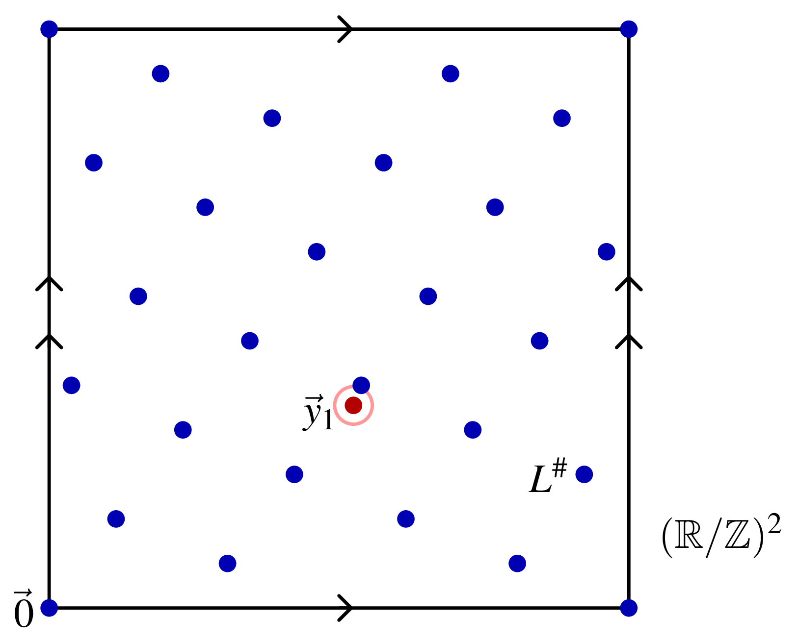
I’ll now let \(G = \mathbb{Z}^d\) and make things more explicit, for starters by putting arrows on elements \(\vec{x} \in \mathbb{Z}^d\) to indicate that they are lattice vectors. The standard begining produces a superposition \(|\psi_{L+\vec{v}}\rangle\) on a translate \(L+\vec{v}\) of the hidden lattice \(L\). (Again, \(L\) is the periodicity of \(f\).) If this state could be an equal superposition on the infinite set \(L+\vec{v}\), and if you could do a perfect QFT on the infinite group \(\mathbb{Z}^d\), then the resulting Fourier mode would be a randomly chosen element of a certain dual group \(L^\# \subseteq (\mathbb{R}/\mathbb{Z})^d\) inside the torus of Fourier modes of \(\mathbb{Z}^d\). Namely, \(L^\#\) consists of those vectors \(\vec{y} \in (\mathbb{R}/\mathbb{Z})^d\) whose such that the dot product \(\vec{x} \cdot \vec{y}\) is an integer for every \(\vec{x} \in L\). (If you expected the Fourier dual of the integers \(\mathbb{Z}\) to be a circle \(\mathbb{R}/2\pi\mathbb{Z}\) of length \(2\pi\), I found it convenient here to rescale it to a circle \(\mathbb{R}/\mathbb{Z}\) of length 1. This is often considered gauche these days, like using \(h\) instead of \(\hbar\) in quantum mechanics, but in context it’s okay.) In principle, you can learn \(L^\#\) from sampling it, and then learn \(L\) from \(L^\#\). Happily, the unknown and irrelevant translation vector \(\vec{v}\) is erased in this method.
In practice, it’s not so simple. As before, you cannot actually make an equal superposition on all of \(L+\vec{v}\), but only trimmed to a box \(B \subseteq \mathbb{Z}^d\). If you have \(q\) qubits available for each coordinate of \(\mathbb{Z}^d\), then \(B\) might be a \(d\)-dimensional cube with \(Q = 2^q\) lattice points in each direction. Following Peter Shor’s famous paper, the standard thing to do here is to identify \(B\) with the finite group \((\mathbb{Z}/Q)^d\) and do the QFT there instead. This is gauche as pure mathematics, but it’s reasonable as computer science. In any case, it works, but it comes at a price. You should rescale the resulting Fourier mode \(\vec{y} \in (\mathbb{Z}/Q)^d\) as \(\vec{y}_1 = \vec{y}/Q\) to match it to the torus \((\mathbb{R}/\mathbb{Z})^d\). Even if you do that, \(\vec{y}_1\) is not actually a uniformly random element of \(L^\#\), but rather a noisy, discretized approximation of one.
In Shor’s algorithm, the remaining work is often interpreted as the post-climax. In this case \(L = p\mathbb{Z}\), where \(p\) is the hidden period of \(f\), and \(L^\#\) consists of the multiples of \(1/p\) in \(\mathbb{R}/\mathbb{Z}\). The Fourier mode \(y_1\) (skipping the arrow since we are in one dimension) is an approximation to some fraction \(r/p\) with roughly \(q\) binary digits of precision. (\(y_1\) is often but not always the very best binary approximation to \(r/p\) with the available precision.) If you have enough precision, you can learn a fraction from its digits, either in base 2 or in any base. For instance, if I’m thinking of a fraction that is approximately 0.2857, then 2/7 is much closer than any other fraction with a one-digit denominator. As many people know, and as Shor explained in his paper, continued fractions are an efficient and optimal algorithm for this in larger cases.
The Shor-Kitaev algorithm works the same way. You can denoise each coordinate of each Fourier example \(\vec{y}_1\) with the continued fraction algorithm to obtain an exact element \(\vec{y}_0 \in L^\#\). You can learn \(L^\#\) with a polynomial number of samples, and then learn \(L\) from that with integer linear algebra. However, this approach can only work if \(L^\#\) is a finite group, or equivalently when \(L\) has maximum rank \(d\). This condition is explicitly stated in Kitaev’s paper, and in most but not all of the papers and books that cite this algorithm. if \(L\) has maximum rank, then the picture in Fourier space looks like this:
However, if \(L\) has rank \(\ell < d\), then \(L^\#\) is a pattern of \((k-\ell)\)-dimensional stripes, like this instead:
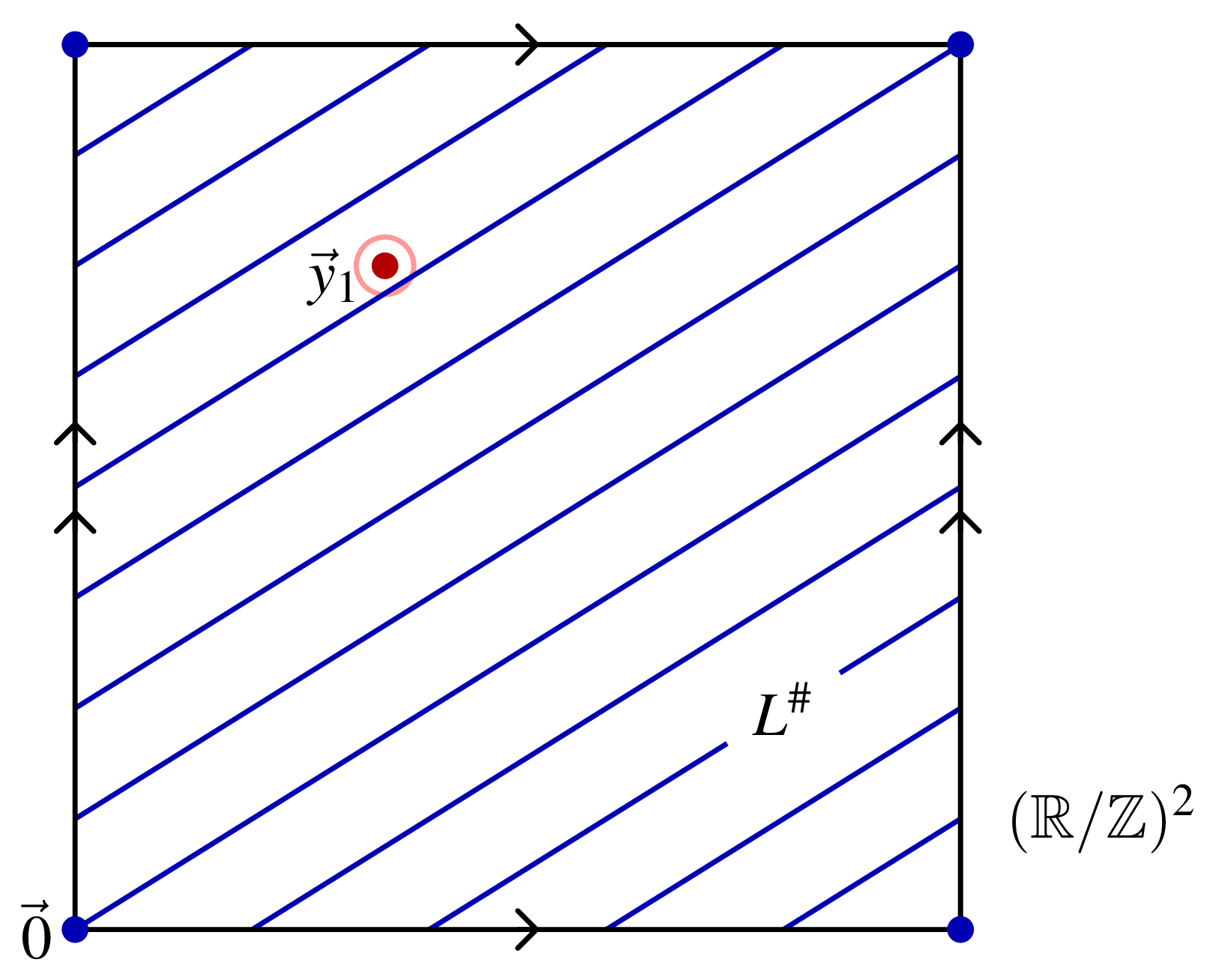
In this case, as the picture indicates, each coordinate of \(\vec{y}_1\) is flat random and individually irreparable. If you knew the direction of the stripes, then you use could define a slanted coordinate system where some of the coordinates of \(\vec{y}_1\) could be repaired. But the tangent directions of \(L^\#\) essentially beg the question. They are the orthogonal space of \(L_\mathbb{R}\), the vector space subtended by the hidden subgroup \(L\). If you know \(L_\mathbb{R}\), then you can find \(L\) by running Shor-Kitaev in the lattice \(L_\mathbb{R} \cap \mathbb{Z}^d\).
My solution to this conundrum is to observe that the multiples of a randomly chosen point \(\vec{y}_0\) in \(L^\#\) have a good chance of filling out \(L^\#\) adequately well, in particular to land near \(\vec{0}\) often enough to reveal the tangent directions of \(L^\#\). You have to make do with a noisy sample \(\vec{y}_1\) instead, but by making the QFT radix \(Q\) large enough, you can reduce the noise well enough for this to work. Still, even if you know that these small, high-quality multiples of \(\vec{y}_1\) exist, they are needles in an exponential haystack of bad multiples, so how do you find them? It turns out that the versatile LLL algorithm, which finds a basis of short vectors in a lattice, can be used here. The multiples of \(\vec{y}_0\) (say, for simplicity) aren’t a lattice, they are a dense orbit in \(L^\#\) or part of it. However, they are a shadow of a lattice one dimension higher, that you can supply to the LLL algorithm. This step produces lets you compute the linear span \(L_\mathbb{R}\) of \(L\) from its perpendicular space, and then as mentioned you can use Shor-Kitaev to learn the exact geometry of \(L\).
 Follow
Comment #1 December 7th, 2020 at 12:34 am
Just like no one in the 1950s foresaw how laser technology could be applied so creatively, this is one small step in showing how even low qubit (100s) quantum computing technology might have unexpected possibilities…
Comment #2 December 7th, 2020 at 2:01 am
Wouldn’t it be historically more accurate to trace the origins of HSP to Simon’s algorithm?
Comment #3 December 7th, 2020 at 9:13 am
Ilya #2 – Well, both Shor and Simon. The two papers came out very close to each other.
Comment #4 December 8th, 2020 at 9:06 am
> Most of the later work has been in the special case that the ambient group G is finite,
Is that because that case comes up if you try to break public key cryptography based on elliptic curves using a quantum computer?
Comment #5 December 8th, 2020 at 12:24 pm
b_jonas #4 – In my opinion, a lot of the work on the hidden subgroup problem has stuck with finite groups largely because that case is mathematically cleaner. That’s not necessarily a wise reason to go that route; you can call it “looking under the streetlamp”. The method in Shor’s algorithm (and in these extensions that I discuss) is to approximate the QFT for an infinite group with a QFT for a finite group. There are infinite groups for which that’s not possible; even when it is possible, it’s messy. It’s a relief to be able to directly equate the QFT you compute with the QFT that you need.
The relevance to elliptic curve cryptography depends on the specific way that you use elliptic curves. The existing elliptic curve cryptography standards are wiped out by Shor’s algorithm, for one thing. In that context, you can calculate the cardinality of the elliptic curve using Schoof’s algorithm. You can then use a version of Shor’s algorithm (or Shor-Kitaev) adapted to that finite abelian group, so that it would more resemble Simon’s algorithm. But since you have Shor-Kitaev for infinite abelian groups anyway, it is sufficient to cite that at least for a theoretical victory.
Now, since then there has been discussion of using my algortihm (for DHSP, not the algorithm here) for cryptography with elliptic curve isogenies. Indeed I looked under the streetlamp too; I set up my algorithm for finite dihedral groups in my original paper. However, there are also versions of my algorithm directly set up for infinite dihedral groups — they are just messier — but for all I know they are better-tuned for applications like this isogeny thing.
Comment #6 December 8th, 2020 at 4:34 pm
Would a stronger generalization of Shor’s algorithm be a step closer to P != BQP?
Not that things seem to work that way – are big results ever iterative? – but that still strikes me as one of the more likely paths.
These are well defined problems, with a well understood quantum speedup that’s not dependent on enumerating a long list of amplitudes.
Comment #7 December 8th, 2020 at 6:55 pm
Job #6: I’m not sure what you’re asking for. People have been trying to generalize Shor’s algorithm ever since it was discovered, with scattered successes, and this post is very much in that direction. But to prove P≠BQP, it’s not enough to find more algorithms—we’d also need to get a hell of a lot better at separating complexity classes.
Incidentally, you can give versions of BosonSampling and Random Circuit Sampling that are every bit as well-defined as factoring is. Whatever other criticism someone has of sampling-based quantum supremacy tasks, that isn’t the issue at all with them.
Comment #8 December 8th, 2020 at 7:13 pm
Job #6 – At one level, separating P from BQP is seen as a cosmically difficult open problem for which any of these algorithms only scratch the surface. At another level, the original Shor’s algorithm already does the job quite nicely, albeit only by a standard (namely oracle separation) that was previously achieved by Bernstein and Vazirani.
The main progress so far in the notorious P vs NP problem consists of barrier results, i.e., how not to prove the conjecture that they are unequal. These barrier results also apply to P vs PSPACE. Then as well, BQP and NP are both contained in QMA, which is thought to be significantly larger; QMA is in PP, which is thought be yet larger; and PP is in PSPACE, which is thought to be very large. The upshot is that even much more generous questions as seen as well out of reach.
On the other hand, the hidden subgroup problem can be cast as an oracle problem; you can make the hiding function an oracle. Then you are sort-of separating P (and BPP) from BQP, except that actually the separation is that BQPf is larger than Pf (and BPPf). The particular way that an oracle is used here (and the examples such as factoring integers and discrete log) is seen as evidence that BQP is indeed larger. Unfortunately, there are also artificial oracle separations that, for instance, make BPP look bigger than P, even though the conjecture is that they are equal with no oracle.
Comment #9 December 9th, 2020 at 12:24 am
Honestly, it wasn’t meant as criticism.
What i mean is that the quantum speedup in period-finding seems more concise than with simulation, where classical algorithms end up solving the related problem of explicitly computing and then sampling from a probability distribution.
With a problem like period-finding, the quantum speedup is right on the surface.
Naively, that seems like better grounds for a separation – there’s less room for classical improvements.
Comment #10 December 9th, 2020 at 10:00 am
Job #9 – It’s true that an exponential quantum speedup for an algebraic problem such as HSP is very crisp and is a great victory on paper. That’s why Shor’s algorithm once captured headlines — and going past the headlines, it directly instigated the very important post-quantum cryptography research program. However, quantum supremacy is capturing headlines now for its own good reason, namely, “A bird in the hand is worth two in the bush.”
The complexity status of random quantum circuit sampling is firmer than you indicate here. Scott and other CS theorists in his circle knew from the beginning that the correct classical foil is any classical algorithm that produces a statistically close sampling distribution, and not necessarily one that computes the distribution and then samples from it. Many of the partial results and lemmas along the way concern computing or estimating values in the distribution, but there is accumulated evidence that satisfactory sampling itself is out of reach for classical computers. Then as well on the algorithm side, the door is open to a sampling method that doesn’t necessarily compute the distribution first. Some of the key strategies do compute the distribution first, but I’m not sure that all of them do — I guess I don’t know the answer to that.
Comment #11 December 9th, 2020 at 10:06 am
Greg Kuperberg #8
The fact that \( BQP \subseteq P^{\#P} \) seems to me to be more interesting than the containments you mention because NP and #P are so similar. I mean that in the sense that if you were told that there was a P-time algorithm for an NP-complete problem, without being given any additional information about it, you would probably have to give a significant probability to a P-time algorithm also existing for #P. I don’t think the same can be said for PSPACE (though I may be wrong, given that I have little familiarity with PSPACE-complete problems).
Comment #12 December 9th, 2020 at 10:12 am
Greg Kuperberg
> f is now periodic with respect to a lattice
How exactly do you define “periodic with respect to a lattice”.
Is this like f(x,y) = sin(x + y) where the function is periodic in both x and y ? If that’s the case I don’t understand why the higher dimensional period finding problem doesn’t trivially reduce to the single dimensional problem where you just set all of the variables but one to some constant.
Comment #13 December 9th, 2020 at 11:45 am
Gerard #11 – The class PP is even more similar to NP than #P is. You can exemplify NP with a question such as “Does this combinatorial jigsaw puzzle have at least one solution?” PP is then “Does it have at least a trillion solutions?”, while #P is “Exactly how many solutions does it have?” PP is clearly a bridge between NP and #P, and conveniently at the formal level, it is a decision problem. You’re right that P#P is another decision problem conversion of #P, but it is probably quite a bit larger than PP. The result that BQP ⊆ QMA ⊆ PostBQP = PP is much sharper than the result that BQP ⊆ P#P.
Meanwhile PSPACE is thought to be truly stratospheric even compared to the others that I mentioned. Its role here is that if we can’t even prove that P ≠ PSPACE, if all we have is barrier results for how not to prove even that, then we might be completely unready to tackle P vs NP or BQP. But note that PSPACE has several alternate definitions that make it look more like NP. NP is a model of perfect-information solitaire games such as Sudoku, jigsaw puzzles, etc. PSPACE equals both AP and IP. AP is a model of perfect-information, polynomial-length two player games such as Othello, chess with a polynomial limit on moves, etc. Meanwhile IP is also a model of solitaire, but this time with randomness or hidden information, e.g., Minesweeper, Klondike, Shanghai, etc.
The hypothesis that P = NP is so outlandish to me that I can’t speculate as to what would happen after that. However, note that you can make an oracle f such that Pf = NPf while PPf is very large. If your intuition is meant to extend to computation with oracles, then Pf = NPf doesn’t necessarily win you a polynomial-time algorithm for #Pf.
By the way, oracles themselves also have a natural game-theoretic interpretation. For instance, NPf is a model of a perfect-information solitaire game that depends on an ad hoc reference database; for example, a crossword puzzle. (Except that as with Scrabble, you would want a rigorous allowed word list, rigorous meanings for the clues, etc.)
Comment #14 December 9th, 2020 at 12:10 pm
Gerard #12 – The hiding function in Shor’s algorithm and the variations that I discuss takes integer inputs, and is best understood as taking values in meaningless symbols. Your proposed example \(f(x,y) = \sin (x+y)\) is partly valid for the problem that I solved. However, (a) you should be thinking \(f(x,y) = h(\sin (x+y))\), where \(h\) is a cryptographic hash function; and (b) the period in this case is very easy, it is just \((1,-1)\). A more illustrative example of the problem that my quantum algorithm solves is
\[ f(x,y) =h(\sin (\frac{x}{12348230087468376}-\frac{y}{3019283742640239871})), \]
where the integer parameters are kept black-box secret from the algorithm, and the sine is evaluated in radians to kill the second period. Moreover, this is just in 2 dimensions. You should now imagine the same sort of problem in (say) 100 integer variables rather than 2, moreover with irrational coefficients chosen so that there is only a single periodic direction.
The Shor-Kitaev algorithm does the same thing, except with the restriction that you have as many directions of periodicity as you have variables. In 2 dimensions, Shor-Kitaev can handle things like \(f(x,y) = h(\sin (\pi(ax+by)))\), where \(a\) and \(b\) are hidden rational numbers.
Comment #15 December 9th, 2020 at 2:51 pm
Greg Kuperberg #13
> If your intuition is meant to extend to computation with oracles
Probably not. My intuition is that a P-time algorithm for an NP-complete problem means that you have found a new way to characterize the solution set of that problem, to the extent of distinguishing an empty set from a non-empty set. Once you’ve made that leap, which for some reason many people seem to find implausible, it seems like a much smaller leap to being able to characterize the solution set so accurately as to be able to determine its cardinality. It’s not clear to me how oracles would affect that argument.
As for PP, I don’t know much about that or other probabilistic complexity classes because I still think that it’s entirely possible that a deterministic P-time algorithm for an NP-complete problem exists and that seems like a much more valuable path to pursue.
There’s something that confuses me though. You say that PP = PostBQP and according to the graph in the header to this website \( NP \subseteq PostBQP \). However the complexity zoo defines PP this way:
> The class of decision problems solvable by an NP machine such that
> If the answer is ‘yes’ then at least 1/2 of computation paths accept.
> If the answer is ‘no’ then less than 1/2 of computation paths accept.
So isn’t it explicitly defined as a subset of NP, not a superset ?
Comment #16 December 9th, 2020 at 3:30 pm
Greg Kuperberg: thank you for the replies, I like those analogies.
Comment #17 December 9th, 2020 at 5:10 pm
Gerard #15 – In the role that oracles play in computational complexity, it is not enough to not know whether oracles would affect a proposed argument or an intuitive expectation. Even though oracles can be deeply artificial, only a minority of known, viable ideas in complexity theory are affected by the presence of an oracle. Most of computational complexity theory is oracle-independent, which is to say it relativizes. Moreover, non-relativizing arguments tend to be more clever, more delicate, or both. If you have ideas or even opinions about a non-relativizing question like P vs NP, then you’re probably not avoiding the oracle issue unless you know a reason that you are avoiding it.
Even though PP is named as “probabilistic” polynomial time, and even though its standard definition that you quoted is probability-ish, it is much better to think of it as a threshold simplification of #P, and thus a generalization of NP. In other words, if a question is in PP, then it asks, for some function f(x) in functional P computable from the input x, are there at least f(x) accepted certificates? If you set f(x) = 1, then you get NP as a special case. The argument that PP contains NP, which is written nicely in Wikipedia, can be extended to justify this more flexible definition.
Comment #18 December 9th, 2020 at 6:27 pm
Greg Kuperberg: I agree. I think it’s exactly the cryptography angle that convinces me that the complexity class separations are hard because they’re non-relativizing.
Symmetric cryptography is based on our belief that there are trapdoor permutation functions that we can compute in a polynomial time, but it’s impossible to compute their inverse in a polynomial time. If we could prove that such functions exist, that would more or less prove that P != NP. But nobody knows how we would even start to prove this. To add to the injury, we also don’t really know how to make an algorithm that implements what we can reasonably conjecture is a trapdoor function in polynomial time. Instead we make do with trapdoor functions where we conjecture that nobody will find a fast algorithm for the inverse within twenty years, and we don’t have a general recipe for this either, instead the best cryptographers collectively invent such a function every few years based each time on entirely new principles. But if you only want to prove a relativizing version of P != NP, it’s much easier. Then it’s enough to imagine an oracle that, for every n, somehow remembers a random permutation of the length n strings. If you had such an oracle, you could use it as a trapdoor function that would enable unbreakable symmetric cryptography: having access to the oracle doesn’t help you to compute its inverse function. But of course that oracle can’t be in P, or even in P/poly, so this doesn’t help us do efficient cryptography in the unrelativized real world.
Something similar but more restricted can be said about BPP != BQP. Here we may use the hidden subgroup problem. Suppose that for each n, finite groups of size (approximately) 2**n, their elements represented as strings of length n (up to some bound), we can compute the group product on those representations in polynomial time, but nobody can compute the group inverse of random elements in randomized polynomial time. We could use this group product function as a primitive for public key cryptography. And, as Greg Kupenberg reminds us here, with Shor’s algorithm a quantum computer could compute the group inverse efficiently, thus proving BPP != BQP. We have candidates for such a hidden group product algorithm based on integer discrete logarithm and elliptic curves that we use in cryptography, but we’re not really sure that the inverse really can’t be computed in classical polynomial time, or how to prove anything like that. For the relativized version, imagine an oracle that, for each n, remembers a hidden random encoding of some easy finite group of size around 2**n to strings, and computes group product using that. Such an oracle would let us do unbreakable public key cryptography if used correctly, because even if the attacker has access to the oracle, it doesn’t help them compute the group inverse efficiently. But the random encoding and its inverse can’t be computed efficiently, so this oracle can’t be in P, or even in P/poly. And to add insult to injury, if we used an efficient algorithm to compute the encoding of the group and its inverse, then the attacker could use that algorithm to compute the group inverse, so we still couldn’t use this method for public key cryptography. The oracle only gets away with it because it’s a black box, there’s no way to ask it to compute just the group encoding or its inverse and tell the result. Admittedly the analogy in this case is worse. It’s possible to imagine that such an efficient to compute hidden group product algorithm does not exist, yet BPP != BQP for some other reason. And there are probably ways to implement public key cryptography without a hidden group product, in such ways that can’t be broken with a quantum computer and so don’t let you prove BPP != BQP.
Comment #19 December 9th, 2020 at 7:22 pm
Greg Kuperberg #17
> In the role that oracles play in computational complexity, it is not enough to not know whether oracles would affect a proposed argument or an intuitive expectation.
Though I’m aware that relativization has been used to exclude a number of ideas for proving that P != NP, I have never heard of a case of it being used against an idea for a P-time algorithm for 3-SAT (for example) and I have trouble seeing how it could be. To prove that P = NP you just have to find an efficient algorithm for some specific NP-complete problem (such as 3-SAT), not one for a whole family of “related” problems (3-SATA \( \forall A \)).
Comment #20 December 9th, 2020 at 8:20 pm
Greg Kuperberg #17
After thinking some more about your definition of PP it seems to me that:
1) The complexity zoo’s definition is poorly worded.
2) PP is “essentially the same” as #P. I mean this in the sense that, even restricting f(x) to a constant, one can compute the exact cardinality of the solution set with a polynomial number of calls to a PP oracle, in the same way that one can compute a solution (ie. certificate) to an NP problem with a polynomial number of calls to an NP decision oracle. I think the way to express this in complexity theoretic notation is perhaps \( FP^{PP} = \#P \).
Comment #21 December 9th, 2020 at 9:47 pm
Gerard #19 and #20 – Okay, I’m speaking a little loosely in discussing the strength of the relativization barrier. I’ll concede one point, that relativization is more convincing as a barrier to showing that P ≠ NP than as a barrier to showing that P = NP. But concerning why people believe so strongly that P ≠ NP, I’ll just say that I personally understand CS theory and a lot of mathematics a lot better believing that P ≠ NP than believing that they are equal. My only temptation to believe that they are equal would be to set up a mental fight between P = NP and P ≠ NP in an effort to solve the Millennium Prize problem. Still, at least CircuitSAT does have a relative version in which oracle calls are allowed as gates. Some of the naive proposed algorithms to show that P = NP are almost as “likely” to work for CircuitSATf with oracle gates as for standard 3-SAT. I admit that that’s a snarky comment, since for many oracles you can flat-out prove that CircuitSATf is not in Pf.
Concerning #P vs PP, actually the Complexity Zoo states as an exercise for the reader that P#P = PPP. The proof is what you’ve intuited, that FPPP contains #P because you can play high-low. Still, naked #P is probably much smaller than FP#P for various reasons. For instance, a problem in #P can only report an answer of 0 when the predicate has no solutions, i.e., corresponding to a problem in coNP. But a problem in FP#P can report an answer of 0 for all kinds of reasons other than that one. For instance, it can report 0 when the predicate has an even number of solutions, which is a very different criterion.
Comment #22 December 9th, 2020 at 10:36 pm
Greg Kuperberg #21
Yes, I agree that PPP = P#P is the correct statement instead of what I had written.
It feels a bit cumbersome though for describing two classes that are mutually P-time reducible to each other. One almost wants to write something like \( PP \approx \#P \) to indicate that two classes are equivalent except for the form of their outputs..
Comment #23 December 10th, 2020 at 2:33 am
Factoring is interesting in that, even if we can’t factor an arbitrary n-bit number in O(n^k) time, we can definitely factor all 2^n n-bit numbers in O(2^n * n^k) time, for any n.
Is that also true for NP-Complete problems? That seems plausible, but less obvious.
It’s basically about the complexity of generating every possible problem-solution pair.
Are there “bulk” versions of complexity classes like P, NP, etc?
I wonder what kind of problems are not in “bulk-P”.
Comment #24 December 10th, 2020 at 8:32 am
This is an offtopic question for Scott or anyone about circuit bounds and P/poly:
I ran across a theorem by Kannan that can be stated as follows:
> For any integer k, there are languages in the PH with circuit complexity nk.
Does this not imply that \( PH \not\subseteq P/poly \) ?
If so then why isn’t that sufficient to prove P != NP via the following argument ?
> If P = NP then PH = P, but \( P \subseteq P/poly \) therefore \( P = NP \Rightarrow PH \subseteq P/poly \) which contradicts the above theorem.
My guess is that there’s something about the definition of P/poly that I’m not really understanding.
Comment #25 December 10th, 2020 at 2:44 pm
Gerard #22 and #24 – Mutual Turing-Cook reduciblility is a perfectly reasonable equivalence relation between complexity classes that people should definitely keep in mind. Although the standard notation is PA = PB, you could just as well write it as something like A ~P B. Only people should keep in mind that it is not the same thing as equality of complexity classes. (I’ve seen people who ought to know better lose track of that point.) Obviously NP and coNP are equivalent in this sense, but NP ≠ coNP is an important refinement of P ≠ NP, part of the larger conjecture that PH does not collapse.
The reason that Kannan’s theorem does not prove that P ≠ NP is the order of the quantifiers. (See page 3 of Luca Trevisan’s notes.) His theorem is that for every polynomial p(n), there is a decision problem d(x) in PH (indeed in Σ2P) with circuit complexity Ω(p(n)). But for your remark to work, d would need to be independent of p, i.e., that there is an d(x) such that for every p(n), the circuit complexity is Ω(p(n)).
Indeed, the real thrust of Kannan’s theorem is that it applies to a non-uniform family of circuits. Your remark only needs the time complexity to be Ω(p(n)), not the circuit complexity. Then you can actually do better than Kannan’s theorem: For every polynomial p(n), there is a decision problem d(x) in P (ordinary P, not PH!) with time complexity Ω(p(n)). This is just the Hartmanis-Stearns time hierarchy theorem, the celebrated 1960s result that helped give birth to computational complexity theory. As Luca Trevisan remarks, this does not yield a proof that P ≠ P.
Comment #26 January 4th, 2021 at 11:21 pm
I hope you’ll forgive me for asking here; comments are closed on the May 20th post with the link to your lecture notes. I’m trying to learn QM and QC in my retirement, and I found your lecture notes valuable. I’m stuck on equation 2.3, though. Is it a typo? Should the plus sign second from the right be an equals sign? Or do all four terms really sum?
Happy new year, regards, and thanks again for making those notes available.
Comment #27 January 4th, 2021 at 11:59 pm
Okay, I see that the four terms are right for the math to work, but I don’t understand where the conjugates came from in the last two terms. I don’t see how they got there from equation 2.1, that’s my confusion.
Comment #28 January 5th, 2021 at 12:58 am
Ward Smythe: Do you understand that |x|2 = xx* ? (If not, check it.)
So then |x+y|2 = (x+y)(x*+y*) = xx* + yy* + xy* + yx*.
Comment #29 January 5th, 2021 at 10:23 am
Ah, the light bulb lights, thank you. That step [to (x+y)(x*+y*)] was my blind spot. In school my math only went as far as limits and derivatives, so I’m playing catch up big time. Watching lots of math and QM videos and reading sources, but at my age learning isn’t as easy as it used to be. I appreciate your help with such a simple question!
Indeed, I’m greatly indebted to you and many others who still believe the internet is a place for freely sharing information and one’s work. Thank you very much!